Summary of the GAMES101 Series (4) - How to Apply Texture Mapping

上一篇关于Shading的博客中最后我们提到了Texture是我们用来对点进行输入的方式。

Before we said, each point has its own UV coordinates, and then find the corresponding point on the map through the UV coordinates, and then take out the value. We can interpolate the pixels in the middle of the triangle through the center coordinates.

But the problem is, if our map is too small, it may cause the model to have multiple points corresponding to the same UV, which will cause blurring. On the contrary, if the map is too large and the UV coordinate difference is too large, it will cause the final jagged or moiré effect.

This article will talk about how game engines solve these two problems.

Basic sampling rules

(X, y) are the pixel coordinates on the screen, (u, v) are the texture coordinates corresponding to the points on the model

for each rasterized screen sample (x,y): 
    (u,v) = evaluate texture coordinate at (x,y) 
    texcolor = texture.sample(u,v);
    set sample’s color to texcolor;

What happens if the sticker is too small

Solution 1: Texture enlargement

This scheme is the simplest scheme, the texture is too small to be enlarged by a certain algorithm.

Here we introduce a new concept called texel, which is a pixel on a texture, and our UV coordinates take a texel from the texture

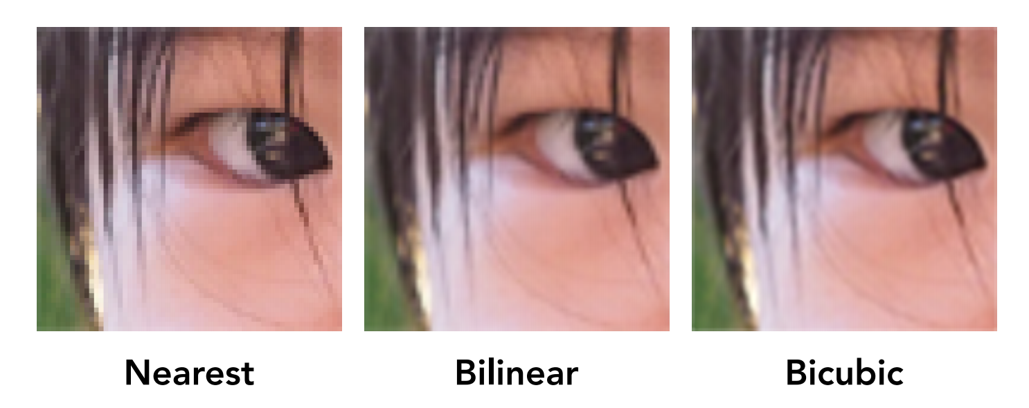
There are three common algorithms for texture amplification: Nearest, Biliner, Bicubic

Let’s take Biliner as an example to explain the process of texture enlargement.

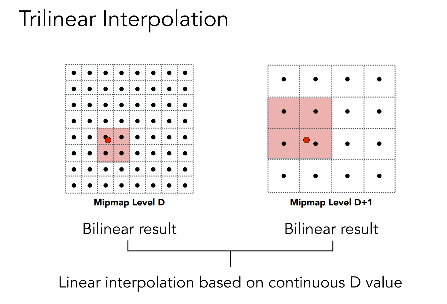
Suppose we want to sample the value of the red point in the following figure, we select four points around the point, then calculate the distance between the point we want to sample and the center of the four texels, and interpolate with this distance:

What happens if the texture is too large

First, let’s look at a rendering:

In the near place, because the texture is too large, some details are lost, resulting in jagged teeth, while in the distance, molar patterns are produced due to too many details. (The reason belongs to personal understanding, but the effect is right)

When the texture is too large, it actually has the following effect:

That is, when we use the “basic sampling rule” mentioned at the beginning to find a certain textured element on the map, we find not one, but a piece.

In other words, if the texture is too small, multiple pixels will find the same texel, and if the texture is too large, one pixel can match multiple texels

Option 1: Supersampling

The algorithm of this oversampling technique is actually the same as the texture amplification just now, but for the case of too small a texture, oversampling is aimed at the original map, which is used to generate a higher resolution original map, and when the map is too large, A pixel may correspond to multiple texels, so the sampling result of the pixel from the map is jointly determined by multiple texels around it.

The following picture shows the effect of super sampling:

It can be seen that supersampling is indeed effective, but the problem is that the calculation cost is too high, and each pixel needs to calculate the value of multiple points and interpolate.

Option 2: Find the average

Supersampling calculation is troublesome, we can simply average it over a range

Option 3: Mipmap

This is a faster range query, is a kind of space for time idea, we need to calculate the results of the range query at different sampling frequencies in advance and store them in the map, that is, to generate maps with different degrees of low resolution. When the map is too large, go directly to the smaller resolution map to find it.

Mipmap is a texture mapping technique used to render textures with different details at different distances and angles. A Mipmap texture is composed of multiple texture images of different resolutions, each image is 1/4 the size of the previous image. The level of Mipmap refers to the first few images in the Mipmap texture, counting from 0, and 0 is the original texture image.

This plan has two key points:

1. Generate different levels of Mipmap
2. How to determine which level of Mipmap to use

The first point is the image compression algorithm, there are many, we do not go into detail, nor rendering specific knowledge, we mainly look at how to determine the level, that is, the “D”

The level of Mipmap can be calculated using the following formula:

level = log2(max(w, h))

Where w and h are the width and height of the texture image, and max (w, h) represents the maximum value in width and height. This formula means that each Mipmap level image is 1/4 the size of the previous level image, so use the logarithm function to take 2 as the base when calculating, and you can get the size of the largest level.

For example, if the size of the original texture image is 512x512 pixels, the Mipmap texture contains 8 levels, which are level 0 to 7. Level 0 is the original image, level 1 is a 256x256 pixel image, level 2 is a 128x128 pixel image, and so on.

We need to use a reasonable Level to have a good price comparison effect. The higher the level, the less details. If we use the oversampling method with too little texture, it will be more blurry:

Plan 4: Anisotropic

Mipmap actually has limitations, it can only do mipmap on textures in the positive direction.

Because of his limitation, on the one hand, when sampling, many unused points will be used, increasing the amount of calculation, and secondly, some pixels correspond to rectangles covering multiple texels, resulting in oversampling blur.

For the case of rectangles, we can use Anisotropic Filtering

Scaled square maps are on the diagonal, other locations store some width compressed and length compressed maps